Introduction

Torch tensors have a slightly different use of the term contiguous. Firstly, let's understand what's contiguous memory is and then we will move on to understanding how torch tensors interpret it.

Contiguous memory VS Non-Contiguous memory

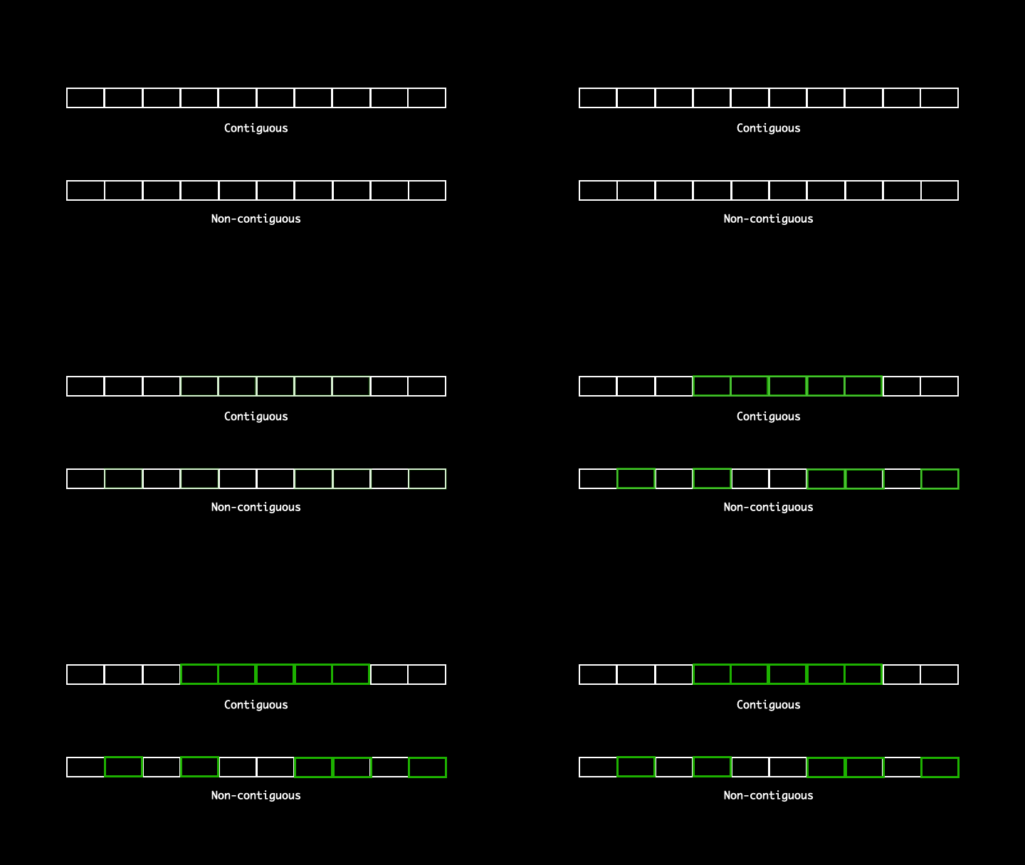
Memory in RAM is distributed for two umbrella processes - 1) Operating System(OS) 2) User Processes. Memory used by OS processes is reserved, the rest of the memory is for user processes, such as launching an application, compiling code, etc. One way to allocate the said memory is through assigning continuous chunks of memory called contiguous memory, rather than allocating dispersed cells.

Contiguous blocks can further be classified to static and dynamic blocks, aka Fixed size partition and Variable size partition, respectively.

torch.Tensor.is_contiguous()

Torch tensors in order to save some compute changes the metadata of the tensor, thus changing the corresponding attributes. There are some interesting observations on stride of the tensor as we explore .transpose() / .T.

In []: x = torch.rand(6, 3)
	   x
Out[]: tensor([[0.9606, 0.5842, 0.4315],
		[0.6616, 0.1583, 0.6887],
		[0.8908, 0.8501, 0.9232],
		[0.3255, 0.7929, 0.8346],
		[0.9268, 0.9570, 0.2518],
		[0.3422, 0.2727, 0.7628]])

In []: x.is_contiguous()
Out[]: True

In []: x.stride()
Out[]: (3, 1)

In []: x.storage().data_ptr()
Out[]: 140576519772288

In []: x[0, 0].data_ptr()
Out[]: 140576519772288

In []: x[0, 1].data_ptr()
Out[]: 140576519772292

In []: x[1, 0].data_ptr()
Out[]: 140576519772300

Stride

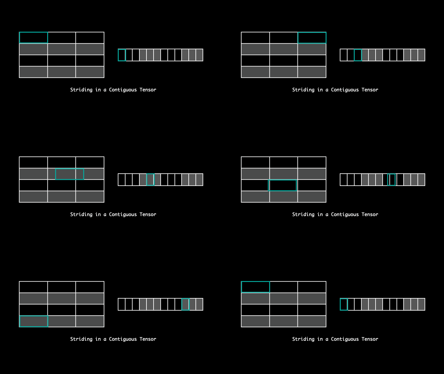
Stride tells us the number of bytes we need to travel to access the following element in a particular direction.

For example, with stride (3, 1), to access the next elements across a row(or in the following column) we will have to travel 1 byte, whereas to access an element across columns(or down to next row) it will move 3 bytes.

This stride pattern changes as we take transpose of the matrix.

In []: x.T
Out[]: tensor([[0.9606, 0.6616, 0.8908, 0.3255, 0.9268, 0.3422],
		[0.5842, 0.1583, 0.8501, 0.7929, 0.9570, 0.2727],
		[0.4315, 0.6887, 0.9232, 0.8346, 0.2518, 0.7628]])

In []: x.T.is_contiguous()
Out[]: False

In []: x.T.stride()
Out[]: (1, 3)

In []: x.T.storage().data_ptr()
Out[]: 140576519772288

In []: x.T[0, 0].data_ptr()
Out[]: 140576519772288

In []: x.T[0, 1].data_ptr()
Out[]: 140576519772300

In []: x.T[1, 0].data_ptr()
Out[]: 140576519772292

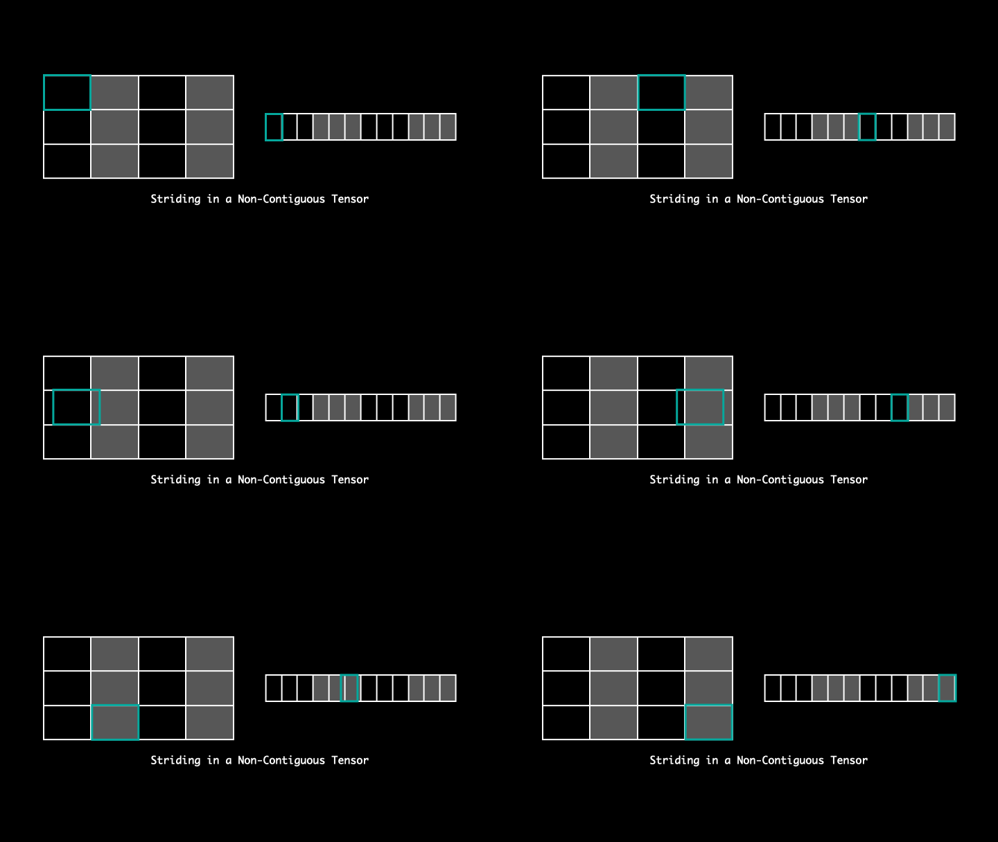
Following the same angle, we can say that the pointer moves 1 step in memory to access the following element along a row and 3 steps to access the adjacent elements down a column.

It's intuitive enough to state that changing the metadata helps us reduce the compute for transpose of the matrix.

⚠️ The memory allocated to the tensor is actually a continuous block, it's just the stride that makes the tensor 'non-contiguous'. Don't let the term mislead you.

Although the elements reside in a continuous block of memory, it's the way they are accessed that makes the tensors non-contiguous. As you can see in the visualisation, the strides are dispersed and the following elements of the tensor along a row isn't the following element in the said memory. Thus, making it non-contiguous. One can readjust the striding by using .contiguous().

In []: x.T.contiguous().stride()
Out[]: (6, 1)

References

https://www.educative.io/edpresso/contiguous-memory
https://stackoverflow.com/questions/48915810/pytorch-what-does-contiguous-do
https://discuss.pytorch.org/t/contigious-vs-non-contigious-tensor/30107/2